I. Introduction

A broad consensus has built up since the early 1990s around the positive role of credit on economic growth, at least at low levels of financial development and under suitable institutional conditions. Featuring one of the least developed banking systems in the world, Haiti stands as a natural candidate to expect credit to become a vital growth engine¹.

This background makes all the more striking the lack of applied research on the sectoral allocation and the effects of private credit on Haiti´s economic performance. As a matter of fact, credit allocation patterns and consequences have been scarcely investigated even for more advanced economies. This study seeks to fill this gap by exploiting for the first time a novel database on credit allocation by industry to produce evidence on the link between overall and sectoral credit and growth in Haiti over the period 2000-2015.

In particular, this document aims to address two research questions: a. How is private credit allocated across sectors in Haiti, and what explains such allocation? And b. Can a meaningful causal link be established between growth and credit by exploiting credit and productive sectoral information? Regarding the first question, it appears that loan portfolios, though diversified, are markedly sticky over time and do not seem to react much to available measures of sectoral risk and return. As for the second question, the econometric work reveals a causal impact of credit on growth at the sectoral level².

The paper is organized as follows. In Section 2 we describe trends on asset composition and loan portfolio allocation across industries in the Haitian banking system. In Section 3 we discuss the theoretical rationale behind bank decisions on loan allocation and we run some econometric exercises to check whether credit flows towards sectors displaying a better recent performance in terms of growth and stability. The core part of the paper, Section 4, tackles the question as to whether credit drives growth in Haiti, beginning with a critical review of the literature on finance and growth in the last quarter century and the severe econometric challenges facing this kind of studies. Subsequently, we adopt and adapt the widely influential Rajan and Zingales’ (1998) methodology on finance-to-growth causality to the Haitian case. Some conclusions and policy recommendations close.

II. An Overall View of Asset and Loan Portfolio Composition of Haitian Banks

Little is known about how banks assign their loans across sectors in Haiti, and many other countries for that matter. This motivates this section on how Haitian banks have been allocated their loan portfolio in the last 16 years, as a preamble to the production of harder evidence on what determines and what effects such allocation has.

To start, Table 1 displays the stylized composition of total bank assets. Three facts stand out. First, based on World Bank data as of 2014, Haiti has a very shallow banking system, with private credit to GDP amounting to just 17.2%, only comparable with other low income countries (18.5%) and well below the levels of other Caribbean nations (40.2%), Latin America (50.6%) or high income OECD countries (122.6%). Institutional weaknesses and macroeconomic instability lie behind this anemic financial intermediation.

Table 1.

Banking System in Haiti: Asset and Credit Composition, 2000-2015

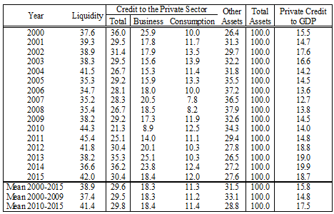
In % of total banking system assets, unless stated otherwise

The second fact is that private credit represents just 29.6% of total assets on average for 2000-2015 without much change over the years. This implies that, for each dollar of funds (from depositors, bondholders and shareholders), only some 30 cents find their way into private credit³. The counterpart is the large liquidity ratio (38.9%) held by banks. In a country with one of the lowest levels of financial intermediation in the world one would have expected most of those resources to meet a presumably large excess demand for credit instead of sitting in the form of liquidity.

This situation hints at both weak supply of and demand for credit⁴. By heightening the default risk of most productive endeavors, Haiti’s volatile and slow economic growth have discouraged the demand for funds by entrepreneurs as well as the willingness of banks to provide financing. In addition, supply is held back by the frail legal creditor rights in place, which makes debt collection in the event of default hard to enforce. More liquidity, despite its lower return vis-à-vis lending, makes for a suitable risk-mitigating buffer stock when banks and firms are reluctant to engage in lending. Last but not least, the regulatory liquidity requirements have been quite high in recent years (indeed well above 40% for both local and foreign currency deposits since 2015), which also explains the low share of credit in bank balance sheets.

The third and last fact highlighted in Table 1 is that household credit has remained around 11% of total assets and 38% of private credit, a lower proportion than the world average (45% according to Beck et al., 2012)⁵.

At the interior of business credit, as shown by Table 2, credit to the services (or tertiary) sector accounts for a staggering 79.8% of total loans on average for 2000-2015. Taking the 2010 earthquake as a turning point for the Haitian economy, the same table shows that this participation has increased, from 78.3% in 2000-2009 up to 82.2% in 2010-2015. According to Table 3, Trade, Restaurants and Hotels appears as the main borrower within the services sector, concentrating 33.7% of all credit. Manufacturing (or secondary) sector takes an average 19.9%, with a declining share from 2000-2009 (21.3%) to 2010-2015 (17.6%). Natural Resources (or Primary Sector) grabs a mere 0.3% of total loans. Distinguishing tradables (Primary and Secondary Sector) from non-tradables (Services), the former have captured an average 20.2% against 79.8% for the latter⁶.

Table 2

Bank Credit Allocation, 2000-2015.

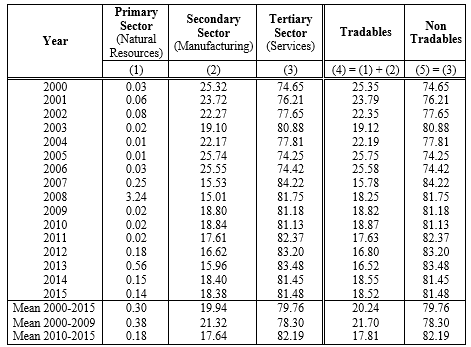
Primary/Secondary/Tertiary and Tradables/Non-Tradables

Table 3

Bank Credit Allocation by Sector, 2000-2015

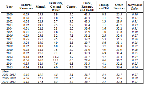
All in all, as attested by the industry shares over time, the loan structure by industry has not changed much over 2000-2015, a phenomenon that raises the question as to how responsive credit allocations are to varying sectoral conditions in terms of asymmetric shocks and relative price changes.⁷ This central question will be dealt with in Section 3 next. Also worth mentioning, the Herfindahl index presented in the last column of Table 3 indicates a reasonably high loan portfolio diversification, an asset in light of the volatile Haitian economic environment.⁸ The index has averaged 0.27 over 2000-2015, even dropping from 0.29 to 0.25 between 2000-2009 and 2010-2015.

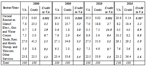
Finally, Table 4 compares the value added (VA) originated by each sector with their participation in total credit. A credit-to-VA higher (lower) than one indicates that a sector is over- (under-) represented in bank loan portfolios⁹. Based on this simple indicator, Electricity, Gas and Water is the most over-represented industry (ratio of 8.9), followed by Manufacturing (2.2). On the contrary, Natural Resources appears to be highly under-represented (0.007), with Transportation and Telecommunications taking the second place (0.5).

Table 4

Share of Sectoral Credit to Share of Sectoral Value Added, 2000-2015

III. Explaining Sectoral Allocation of Credit in Haiti

Having examined the bank loan portfolio composition of Haitian banks, this section aims to explain the observed allocations. At first glance, banks should lend more to those sectors exhibiting a higher expected growth and a lower expected volatility. Nevertheless, the basic principles of financial portfolio construction are not directly applicable to bank loan portfolios, where liquidity and imperfect information aspects gain particular relevance. For one, loans constitute long-term commitments and hence exit via trading is severely limited. Secondly, banks are affected by the well-known problems of adverse selection (that is, distinguishing high and low risk loan applicants) and moral hazard (that is, the borrower’s incentives to lean toward risky projects or refuse to honor their obligations).

As usual, multiple and often contradictory theoretical positions can be found about how banks allocate credit across sectors (see Wurgler, 2000, and Bebczuk and Sangiacomo, 2007). As stated above, the standard view would be that any profit-maximizing and risk-minimizing bank should prioritize in its portfolio the more dynamic and stable sectors. But bank behavior depends on other factors that may turn loan portfolios less or not at all responsive to mere risk-and-return conditions. In the first place, owing to asymmetric information, there might be steep learning costs (and risks) from entering new lending markets and taking previously unknown borrowers. As long as bank managers and shareholders perceived no risk-adjusted gains from making such kind of move, they would prefer sticking to their traditional clientele.

Related to this, some scholars refer to the “lazy banks” hypothesis, positing that banks try to minimize their costs (and managers their effort) by substituting proper borrower screening with collateral and other credit enhancements (see Manove, Padilla and Pagano, 2001). Under this behavioral trait, banks would be even more reluctant to navigate uncharted waters. In the second place, recent observed sector performance may not be a reliable indication of future performance, especially in volatile economies. The same goes for price signals that, when persistent, may lead to portfolio shifts. For instance, a real devaluation should encourage banks to increase their loan share of tradables at the expense of non-tradables, but if markets expect a reversion of the real exchange rate to previous levels in the near future, banks would not act on this signal¹⁰. Thirdly, credit allocation is driven not only by the supply but also the demand for credit. If growing sectors are able to generate retained earnings, their need for credit may be low no matter how willing banks are to serve them.

Finally, loan portfolio stickiness can very well explain by related lending. When unregulated or weakly enforced, as it is the case in Haiti, banks may direct their loanable funds towards firms belonging to the same economic group regardless of their prospects and probability of default.

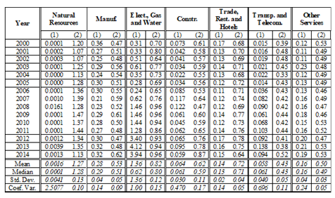
A first, exploratory look at the data appears in Table 5, displaying the mean, standard deviation (SD) and their ratio for each productive sector, accompanied by the respective credit share and its change, with annual data for 2000-2015. A quick test on the link between sector performance and credit access is that sectors with a higher mean and less volatile growth (that is, a higher mean-to-SD ratio) should have experienced a greater increase in their credit share. Table 5 definitely rejects this belief. For example, the sector with the highest mean-to-SD (1.2), Construction, has seen its credit share grow by just 2.8 p.p. (from 4% in 2000-2002 up to 6.8% in 2013-2015), whereas Electricity, Gas and Water, the sector with the next to worst mean-to-SD ratio (0.1) expanded its participation in total loans by 5.8 p.p. (from 2.1% to 7.9%).

Table 5

Loan Portfolio and Value Added Performance by Sector, 2000-2015

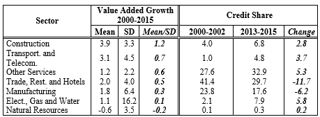
In Descending Order by Mean-to-SD of VA Growth

The econometric exercise in Table 6 boasts a panel regression for our 7-sector, 15-year sample looking to explain the interannual change in the sectoral loan share in year t as a function of the mean and the standard deviation over three years (t to t-2) of the value added real growth¹¹. Neither variable enters significantly, supporting the preliminary evidence about the overall stickiness of loan portfolios to sector-specific conditions. Things do not vary much when we replaced, in Table 7, the mean and standard deviation individual regressors with their ratio.

Table 6

Explaining sectoral credit allocation (I): Industry-level approach

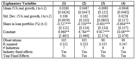
Fixed Effects Estimation, Annual Data for 2000-2015

Robust standard errors in brackets. *** p<0.01, ** p<0.05, * p<0.1.

All equations also include the lagged portfolio share (as opposed to its change) to check whether banks tend to gradually concentrate their lending towards the sectors they have more exposure to and thus know more or, on the contrary, they strive to keep a diversified portfolio and avoid excessive concentration in some sectors¹². The strongly negative and significant coefficient lends credibility to the latter view, which in turn is consistent with the relatively stable portfolio shares unveiled in the previous section and the low and slightly diminishing Herfindahl index.

Table 7

Explaining sectoral credit allocation (II): Industry-level approach

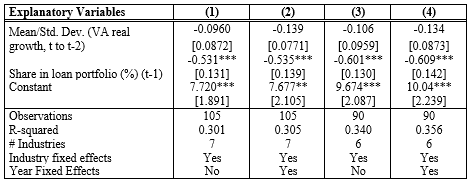
Fixed Effects Estimation, Annual Data for 2000-2015

Robust standard errors in brackets. *** p<0.01, ** p<0.05, * p<0.1.

To close this section, in Table 8 we run a regression for the same dependent variable to identify macroeconomic factors affecting the change in portfolio share at individual industry level using quarterly data¹³. Our main hypothesis is that real devaluations should encourage banks to shift their loan portfolios towards tradable vis-à-vis non-tradable industries, as the former would become more profitable and less prone to default¹⁴. In all, we unearth weak and hardly reliable evidence in favor of this relationship, which is significantly verified at 5% only for Manufacturing (with the expected positive sign) and Construction (negative). Moreover, the economic effect is small: a 10% real devaluation would increase the Manufacturing share in just 0.92 percentage point and would diminish that of Construction in 0.27 pp. Given the macroeconomic nature of the exercise, we also wanted to check, without imposing any particular prior, whether aggregate economic activity influences the loan portfolio composition. Once again, we were unable to detect any significant effect at 5%. On the contrary, as in Table 5, the lagged portfolio share enters negatively and significantly in all cases.

Table 8

Explaining sectoral credit allocation: Macro-level approach

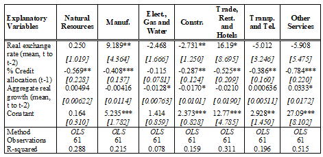
OLS Estimation, Quarterly Data for 2000.Q1-2015.Q4

Robust standard in brackets. ***p<0.01, **p<0.05, *p<0.1

IV. The Effects of Credit on Economic Growth in Haiti: A Sectoral Approach

In sheer contrast to the countless papers on the effects of aggregate credit on aggregate growth, little to none effort has been put into linking sectoral credit and growth¹⁵. In this section, we will explore this issue, building on the scarce existing literature, in the context of Haiti. But first things first, we need to frame this analysis within the broader academic and policy debate around the impact of credit on economic growth.

The causal link between financial development and economic growth remains a highly divisive issue in the academic literature. Prominent economists such as Joan Robinson, in the 1950s, and Robert Lucas, in the 1980s, voiced their skeptical view about any role of finance on growth, contending instead that financial development is just a byproduct of economic development. Then, since the early 1990s a new breed of theoretical and empirical studies forcefully pushed forward the notion that credit was a vital engine of growth (see Levine, 2005). In recent years, in particular in the wake of the 2008 financial deepening on growth (see Panizza, 2013, and Cecchetti and Kharroubi, 2015).

This disconcerting and dynamic debate stems from the fact that causality, unlike basic correlation, is hard to establish. At any rate, we may observe two variables moving in tandem, but that does not provide information on which one causes a change in the other, or whether both are being shifted by a third common driver –the age-old chicken and egg story. Furthermore, in the present case, strong conceptual arguments exist to support either causality nexus. In favor of the credit-to-growth position, researchers underscore the role of the financial system in alleviating intermediation costs and informational barriers between creditors and borrowers paving the way for a more cost-efficient and socially productive allocation of saving. On the opposite camp, scholars claim that the propensity to save may very well explain both financial development (as part of saving is channeled towards the financial system) and economic growth (as saving affects investment, which in turn fosters growth)¹⁶.

At the empirical level, considerable effort has been put into finding sensible instrumental variables to deal with this potential two-way causality and the ensuing endogeneity bias (see Beck, 2009, for a survey on finance-and-growth econometrics). Possibly the most widely accepted method to tackle this issue is the one proposed by Rajan and Zingales (1998) and adopted by leading subsequent studies (e.g., Cecchetti and Kharroubi, op.cit.)¹⁷. Departing from the usual macro-level data analysis, their identification strategy hinges on the sensible hypothesis that productive sectors that are more dependent on external finance (i.e., funds provided by outsiders, as opposed to internal funding via retained earnings) should benefit more from an overall credit expansion than sectors that are less dependent on such resources.

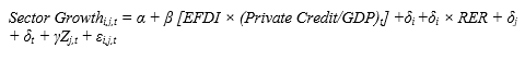
To clearly highlight the underpinnings of this approach, it is helpful to write the stylized version of a typical growth panel regression:

[1]

where the variables δ stand for country (j) and time (t) fixed effects to control for unobservable heterogeneity, and Z is a vector of other time- and country-variant GDP growth drivers.

The main pitfall of this specification is that reverse causality from growth to credit would imply endogeneity, thus rendering the estimated coefficient upward bias. To avoid overestimating the effect of credit on growth, Rajan and Zingales (op.cit.)¹⁸ propose the following general framework:

[2]

where the subscript i denotes industry or sector, and EFDI stands for external financial dependence index. The novelty lies, first, in the choice of an industry-level (as opposite to aggregate or macro-level) dependent variable and, second, a reformulation of the credit regressor. As stated above, the hypothesis is that an expansion of aggregate credit (Private Credit/GDP) would disproportionately boost the growth of the more financially dependent sectors. The underlying assumption is that these sectors have a larger unmet demand for bank credit and other external funding sources, and hence the greater availability of credit should relax such financial constraints and foster industry’s growth¹⁹ .

Measuring financial dependence is not a trivial matter, though. In their multicountry study, Rajan and Zingales (op.cit.) proxy it by the ratio between physical investment minus cash flow (or internal funds) to physical investment, that is, the fraction of physical investment that is financed with external funds in listed U.S. firms, under the assumption that the U.S. is the closest to a frictionless (or perfect) financial market, and so businesses are able to use the optimal amount of external funds. Different sectors may exhibit different financing needs depending for instance on how intensive they are in physical capital and how long the typical product cycle is between launching the project and the actual generation of revenues²⁰.

Domestic financial dependence in each country, say Haiti, may still suffer from endogeneity, as firms in a particular industry may be using little external funding just because they suffer a financial constraint. In such a case, more credit would entail a change in financial dependence, making the latter an endogenous variable and thus a poor indicator of true or intrinsic financial dependence.

Taking the United States as a benchmark would provide, according to these authors, not only an optimal benchmark to assess financial dependence but would also ensure exogeneity, as this index cannot be suspected of being affected by industry or aggregate growth in countries other than the U.S.. By a similar token, growth in individual industries (as opposed to aggregate growth) should not spur aggregate credit growth.

While an undeniably ingenious procedure, we believe, in line with Balta and Nikolov (2013) and Auguste, Bebczuk and Sanchez (2013), some serious caveats weaken the index chosen by Rajan and Zingales (op.cit.), namely:

(a) It is a flow-based (as opposed to a stock-based) measure, and as such it may display high variability over time, which is at odds with the assumed stability of the index²¹ . Investment, cash flow and external funding tend to substantially change over the business cycle and as a result of macroeconomic shocks;

(b) The U.S. financial market, despite being highly developed, is far from frictionless according to the available evidence, meaning that its choice as the optimal benchmark is not obvious.²² This body of empirical work suggests that we cannot be sure that firms worldwide would ideally target the same degree of financial dependence as their American counterparts, which are also subjected to financial constraints, even though of a lesser intensity than in less developed economies. Furthermore, the index is constructed on the basis of listed American firms (only a minor proportion of all firms) in each sector and for a particular set of years in the 1980s, making for a less than fully representative and updated benchmark; and

(c) The index is only calculated for the U.S., assuming as valid, without any evidence at all, the notion that financial dependence is higher and optimal in the U.S. vis-à-vis other economies. In fact, for this methodology to be legitimate, it should be true that for any given industry j, financial dependence is higher in the benchmark country (the U.S. or another country with a well-developed financial system) than in the countries included in the sample (in our case, Haiti).

In order to overcome these pitfalls, our present study will employ the debt-to-value added ratio as the measure of financial dependence, taking several European countries as a benchmark, borrowing data from BACH (2016)²³. The first reason behind the adoption of the stock of outstanding debt (as opposed to the annual flow used in the original index) constitutes a more stable proxy for the use of external funds. Equally important, this index can be reproduced for Haiti for the same industries and years as in Europe, enabling a more fruitful comparison and interpretation that will exploited in our statistical analysis²⁴.

The choice of Europe was determined by the availability of a broad sample of countries (10) and years (2000-2014) for a highly representative sample of listed and non-listed firms. While a highly developed financial market, the average from this European panel is likely to mitigate measurement errors that may stem from the consideration of a single country (the U.S.), outdated figures and a non-representative set of listed companies²⁵.

Table 9 displays the financial dependence index (credit-to-value added) for both Haiti and Europe over the period 2000-2014. The data appears to meet the desirable requirements, i.e.:

• Consistent with the relative development of the financial system, in every single year the financial dependence is notoriously higher in Europe than in Haiti. Comparing mean values, the European ratio exceeds that of Haiti by a factor of 1.9 in Manufacturing, 3.1 in Other Services, 5.3 in Trade, Restaurants and Hotels, 7.4 in Transportation and Telecommunications and 9.8 in Construction. In Natural Resources, due to the low level of credit directed to this sector, the difference is 777 times. The only exception is Electricity, Gas and Water, where financial dependence is 1.36 for Haiti and 0.82 for Europe. The gap in favor of Haiti started in 2008 (1.46 against 0.96) and deepened since 2012, reaching a maximum of 3.94 (compared to 0.96 in Europe) in 2014. The surge in financial dependence in later years is most likely explained by the quest to tackle, through additional bank loans, the structural infrastructure deficit in the country, in turn aggravated by the devastating 2010 earthquake; and

• In both groups, values are reasonably stable over time, with a coefficient of variation (a scale-free dispersion measure equal to the standard deviation divided by the mean) well below one in all sectors but Natural Resources and Electricity, Gas and Water in Haiti, where the statistic exceeds one. These two outliers are easily explained by the facts depicted in (i): in the former case, the relatively high coefficient of variation obeys to the extremely low mean value, whereas in the latter the explanation has to do with the remarkable increase in credit support for infrastructure expansion and reconstruction in recent years²⁶.

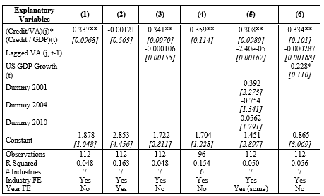
Just to recap, the dependent variable in the following fixed-effects panel estimation is the average annual growth of real value added by industry j. The latter seek to control for unobserved heterogeneity across sectors and over time²⁷ . The main estimations, including the baseline specification as well as several robustness checks, appear in Table 10. As shown in the first row, our variable of interest -Europe’s financial dependence index (measured by the median over 2000-2014) interacted with the credit-to-GDP ratio- delivers in most cases a positive, statistically significant and stable estimate.

In regression (1), the only controls are industry fixed effects (not reported in the table for the sake of brevity). Regression (2) adds year fixed effects. Despite being all non-significant but one, these time effects suppress the explanatory power of the above interaction term and even reverse its sign, so we have tried various alternative control sets²⁸. In column (3) we include the lagged level of value added, intended to (unsuccessfully) capture any conditional convergence –sectors with a larger initial production and presumably capital stock should subsequently grow less than other sectors due to the diminishing marginal productivity of capital.

Regression (4) eliminates the Electricity, Gas and Water sector as a result of its peculiar behavior in terms of credit and negative shocks. Regression (5) reinstates some of the year effects, in particular those corresponding to 2001, 2004 and 2010, that is, the years in which the Haitian experienced negative growth during the whole period 2000-2014. Finally, regression (6) picks up time-variant effects common to all industries –hence a good substitute of year effects- by including the U.S. GDP growth rate²⁹. For our purposes, the key conclusion is that our variable of interest seems for the most part resilient to these stress tests³⁰.

In terms of economic significance, the estimated effect is also noteworthy, and confirms the prior that the sectors more dependent on external funding seem to benefit relatively more from an expansion of aggregate credit. Based on the estimated coefficient in regression (1), if Private Credit to GDP increased from the current 17% to 20%, Transportation and Telecommunications –the least financially dependent sector- would see its average annual growth increase by 0.43 percentage points. Conversely, Natural Resources, the sector with the highest financial dependence, would increase its growth by 1.3 percentage points³¹.

While maintaining the same control sets as in Table 10, Table 11 adopts a different definition for our variable of interest, by replacing average Credit/VA in Europe by the difference in average Credit/VA between Europe and Haiti –what we can call relative (as opposed to the previous absolute) financial dependence. The justification for this change -a novelty in this literature- is to check whether the impact of financial development on industry growth depends not only on the optimal degree of financial dependence but also on distance between it and the industry’s own actual financial dependence.³² A priori, the greater the distance, the more binding the financial constraint, and therefore the more impact a given overall credit expansion should have on industry growth. In the limit, if an industry has already the same financial dependence as the optimal benchmark, changes in credit should not affect their growth.

Table 9

Financial Dependence (Credit-to-Value Added) by Industry Haiti and 10 European Countries, 2000-2014

Source: Own elaboration based on BRH, IHSI and BACH (2016).

Table 10

Industry Growth and (Absolute) Financial Dependence

Panel Estimation with Fixed Effects. Annual Data for 7 Industries over 2000-2015

Robust standard errors in brackets. *** p<0.01, ** p<0.05, * p<0.1.

Based on Table 11, the estimated coefficients do not vary much relative as those uncovered in the regressions from Table 10, but the economic effect of a given credit change is not the same as before. Take the case of Manufacturing, the sector with the shortest distance between the median financial dependence in Europe (0.51) and Haiti (0.29). Under the estimation displayed in column 1, Table 10, a change of Credit/GDP from 17% to 20% would increase its growth by 0.52 percentage points, against 0.23 under the estimation of column 1, Table 11³³. This reformulation does not invalidate, though, the central message of the baseline regressions in Table 10: with the modified regressor, the growth impact for Transportation and Telecommunications would fall to 0.37 down from the previous 0.43, and would remain almost identical (1.29) for Natural Resources, as this sector has an extremely low actual financial dependence in Haiti, and thus the credit effect would be at its maximum.

A major issue in the Haitian economy is the impact of the strong real appreciation of the gourde since the early 1990s, motivated by massive flows of worker remittances and unilateral transfers from abroad. Katz (2015) argues that the decline in Haiti’s GDP per capita is to a great extent explained by such currency appreciation, which has undermined competitiveness in the tradable sector within the manufacturing sector.

Having said that, the relationship between industry growth and the RER cannot be signed as easily due to the disparate effects of a real devaluation (see Bebczuk, Galindo and Panizza, 2010). In a small and open economy, a real devaluation should be most potent in an export-oriented sector with low requirements of imported inputs (and no foreign debt), as in this case the producer may be able to grab the full benefit from the change in relative prices and would also be able to channel the additional production overseas. Conversely, if the sector does not export much but instead sells mostly in the local market, has a high demand for imported productive factors (and/or bears a high foreign debt), the net profit effect for the producer may turn out negative, in which case a real devaluation will become growth-stifling. This negative outcome results not only from the higher costs of foreign inputs and foreign debt payments but also from the lack of exports and the reliance on the domestic market. At the same time that the devaluation improves producer’s profitability, it worsens the local consumers’ purchasing power, determining in some cases that tradable sales would drop rather than increase due to weak internal demand –a phenomenon associated to the so-called contractionary devaluation hypothesis. In sum, the effect of a devaluation is ambiguous a priori.

To delve into the empirics of this question, and since the impact of the real exchange rate (RER) may differ across specific tradable industries, we make use of a breakdown of six activities at the interior of the manufacturing sector (Food and Beverage, Wood, Chemical, Textiles, Paper and Printing, and Other). Table 12 expands on Tables 10 and 11 by adding a new set of regressors. For each manufacturing subsector, a dummy variable was created, and such dummy variable was interacted with the RER. A positive coefficient would indicate that a real gourde appreciation (devaluation) is associated with a lower (higher) value added growth, consistent with the prior that tradable activities thrive with a higher RER and vice versa. Following the previous econometric formulation, the new regression takes the form:

[3]

where RER stands for the real exchange rate.

First of all, we repeat previous exercises by including the same control set and, alternatively, the absolute and the relative financial dependence. In this case, financial dependence remains positive with an even higher value than before, but it is not statistically significant as a result of strong heteroskedasticity in this sample³⁴.

The discussion in previous paragraphs helps interpret the diverging effects of the RER on the performance of manufacturing subsectors. First of all, let us notice that all subsectors identified here, save Textiles, are net importers and only export a minor share -between 0% and 7%- of their total production (see Cicowiez, 2015). Textiles, on the contrary, devotes 58% of its production to international markets and so, even with an import-to-production ratio of 25%, it stands as the sole net exporter in the group. This is likely behind the positive devaluation impact unveiled in all specifications. The opposite case is Food and Beverages, with a negative and significant coefficient, arguably explained by a combination of net imports and a high elasticity of domestic demand (especially by low-income households). Among the other subsectors, we find non-significant effects on Wood and Chemical and a positive and significant one on Paper and Printing and the residual category Other Manufacturing.

In regressions (5) and (6) we go back to the overall manufacturing sector, obtaining a negative and significant effect. A general lesson to draw is that a reversion of the secular gourde appreciation may bring multiple and hard-to-anticipate effects, with both winners and losers not only on the productive but also the income distribution front.

Table 12

Manufacturing Growth and Real Exchange Rate

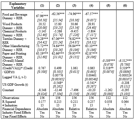
Panel Estimation with Fixed Effects. Annual Data over 2000-2015

V. Conclusions

The present study has examined sectoral credit allocation in the Haitian banking system over the period 2000-2015 and produced fresh evidence on the link between credit and growth at the sectoral level, exploiting for the first time a dataset administered by the Banque de la Republique d’Haiti (BRH).

The main conclusions from our empirical analysis are: (1) While the loan portfolio looks diversified across sectors, credit shares by industry appear to be sticky over time in spite of changing industry-specific conditions and sharp relative price changes, in particular the real exchange rate; (2) Consistent with the previous finding, econometric exercises confirm that loan portfolio allocations are not governed by recent sector performance, casting doubts about the efficiency of loan portfolios; (3) The majority of productive sectors in Haiti seem to suffer from intense financial constraints, as shown by the low use of bank debt compared to advanced economies; and (4) Based on an endogeneity-mitigating methodology, overall credit expansion seems to be a major driver of industry growth.

The chief policy prescription emerging from the analysis is that efforts to stimulate financial intermediation in Haiti should be strengthened, which in turn would require a profound institutional upgrade –in particular, better and more effective creditor legal rights and well-functioning credit registers- coupled with more stable economic conditions. A profuse body of work over the last two decades has produced compelling evidence on the benefits of these institutional improvements in terms of financial deepening (see Djankov, McLeish and Shleifer, 2007).

Equally important, in light of the apparent growth and welfare implications of financial intermediation, more granular data is necessary to evaluate bank decisions at the time of allocating portfolios. For instance, while sectoral data represents a valuable step forward compared to aggregate data, detailed balance sheet and credit information for individual businesses would be greatly welcome. This sort of data would enable to assert whether the current loan distribution is efficient, in the sense that the most promising and dynamic sectors are being rewarded with more access to credit under acceptable conditions of amount, maturity, interest rate and collateral. If that is not the case, corrective policy measures would be in order, led by public banks or through other financial assistance programs. At any rate, these interventions should be carefully designed and monitored, including periodic cost-benefit and impact evaluation analyses.

References

Acharya V., I. Hasan and A. Saunders (2006), Should banks be diversified? Evidence from individual bank loan portfolios. Journal of. Business. Vol. 32, 1355-1412.

Auguste S., R. Bebczuk and G. Sánchez (2013), “Firm Size and Credit in Argentina”, IDB Working Paper No. 396, Inter-American Development Bank.

BACH (2016), Banks for the Accounts of Companies Harmonized, European Committee of Central Balance Sheet Data Offices (ECCBSO), available at http://www.eccbso.org

Balta N. and P. Nikolov (2013), “Financial Dependence and Growth since the Crisis”, Quarterly Report on the Euro Area, Vol. 12, No. 3, European Commission.

Bebczuk R., A. Galindo and U. Panizza (2010), “An Evaluation of the Contrationary Devaluation Hypothesis”, in Esfahani H., G. Facchini and G. Hewings (eds.), Economic Development in Latin America, Palgrave Macmillan. Previously published as Working Paper No. 582, Research Department, Inter-American Development Bank.

Bebczuk R. and M. Sangiácomo (2007), “Eficiencia en la asignación sectorial del crédito en Argentina”, Ensayos Económicos, Vol. 49, Banco Central de la República Argentina.

Bebczuk R. and A. Galindo (2008), Financial crisis and sectoral diversification of Argentine banks, 1999-2004, Applied Financial Economics, Vol. 18, 199-211.

Beck T., B. Buyukkarabacak, F. Rioja and N. Valev (2012), “Who Gets the Credit? And Does It Matter? Household vs. Firm Lending Across Countries”, The B.E. Journal of Macroeconomics, Vol. 12, Issue 1, Article 2.

Buera F. and Y. Shin (2013), “Financial Frictions and the Persistence of History: A Quantitative Exploration”, Journal of Political Economy, Vol. 121, No. 2.

Cecchetti S. and E. Kharroubi (2015), “Why does financial sector growth crowd out real economic growth?”, BIS Working Paper No. 490, Bank of International Settlements.

Chun S., H. Kim and W. Ko (2012), “The Impact of Strengthened Basel III Banking Regulation on Lending Spreads: Comparisons across Countries and Business Models”, mimeo, Bank of Korea.

Cicowiez M. (2015), “A CGE Model for Haiti”, Inter-American Development Bank, November.

Djankov S., C. McLeish and A. Shleifer (2007), “Private Credit in 129 Countries”, Journal of Financial Economics, Vol. 12, No. 2, 77-99.

Fan J., S. Titman and G. Twite (2012), “An International Comparison of Capital Structure and Debt Maturity Choices.” Journal of Financial and Quantitative Analysis 47(1): 23-56.

Jahn N., C. Memmel and A. Pfingsten (2013), “Banks’ concentration versus diversification in the loan portfolio: new evidence from Germany”, Working Paper No. 53/2013, Deustche Bundesbank.

Kadapakkam P., P.C. Kumar and L. Riddick (1998), “The Impact of Cash Flows and Firm Size on Investment: The International Evidence.” Journal of Banking and Finance 22: 293-320.

Katz S. (2015), “¿Podrá, Aiyti, volver a ser el Reino de este Mundo?”, mimeo, Inter-American Development Bank, November.

Levine R. (2005), “Finance and growth: Theory and evidence”, in P. Aghion and S. Durlauf (eds.), Handbook of Economic Growth, Elsevier.

Manove M., A. Padilla and M. Pagano (2001), “Collateral versus Project Screening: A Model of Lazy Banks”, RAND Journal of Economics, The RAND Corporation, 32(4), 726-744, Winter.

Panizza U. (2013), “Financial Development and Economic Growth Known Knowns, Known Unknowns, and Unknown Unknowns”, Working Paper 14/2013, Graduate Institute of International and Development Studies, Geneva.

Rajan R. and L. Zingales (1998), “Financial Dependence and Growth”, American Economic Review, Vol. 88, No. 3, 559-586.

Wurgler J. (2000), “Financial Markets and the allocation of capital”, Journal of Financial Economics, Vol. 87, 187-214.

Notes

Additional information

Clasificación JEL:: O47, O16